
3.3.2 Costs

Costs 

Total cost - the total expense incurred in reaching a particular level of output. 

TC = TFC + TVC 

Total fixed cost - costs that do not vary with output. 
e.g rent, R&D, advertising

Total variable cost - costs that vary with output 
e.g raw materials, labour, power 

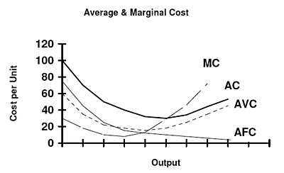
Average (total) cost - the cost in producing a unit output. Obtained through dividing TC by Q (quantity sold). 

ATC = TC/Q
Image result for cost curves

Average fixed cost - fixed cost in producing a unit output. AFC is not fixed - increasing the output spreads the TFC (a fixed quantity) and divides it, making it smaller and reducing the cost per unit output. 

NB: area under the AFC curve is TFC. 

AFC = TFC/Q 

Average variable cost - variable cost per unit output 

AVC = TVC/Q 

Marginal cost - equal to marginal variable cost as there are no marginal fixed costs. 
Image result for cost curves


We define the short run as time in which at least one factor of production is fixed, and the long run as time in which all factors of production are variable. 

i.e in the SR a firm can vary labour and not capital, in LR a firm is able to vary both. 

Law of diminishing returns/diminishing marginal productivity


Diminishing returns occur where the marginal productivity falls. In the SR the presence of a fixed factor can put a constraint on the productivity of the variable factors. 

As you add variable factors of production to a combination containing at least one fixed factor, the productivity of the variable factor will inevitably decline. (though at first it will rise) 

e.g MIVs digging up potatoes(!) 
if there is only a fixed number of shovels, as you employ more MIVs the number of potatoes dug up will at first increase (as the shovels are put to use), and then still increase but at a decreasing rate as all the shovels are used and the extra MIVs are forced to dig with their hands/stand around and do nothing to increase output. 

This explains the parabolic shape of the AC curve - at first productivity increases, so the firms' cost per worker declines. After a certain point, however, the law of diminishing returns kicks in and the cost per worker rises, meaning the AC slopes upwards. 

The TC curve reflects the law too - at first each additional unit doesn't add too much to the cost so the gradient is shallower, but as productivity decreases each additional unit adds more to the total cost and the curve slopes upwards at a steeper gradient. 


Relationship between SRAC and LRAC 

The LRAC shows the minimum possible cost of producing a given level of output with present technology. The firm is limited in the SR to varying output along the SRAC due to a fixed factor of production, and if it changes FoP it moves to a different SRAC. In the LR however, all FoPs are variable, so we get a LRAC that 'envelopes' all the SRAC. The LRAC touches each of the SRAC (not necessarily at their minima though). The SRACs cannot undercut the LRAC because SR costs are never lower than LR costs. 
Image result for LRAC


Comments

Popular posts from this blog

Business Growth

Why do businesses grow?  Profit motive Businesses grow to make more profit by increasing revenue. Selling more to more people often means profits increase.  The valuation of a company's share is often influenced by how it is expected to do in the future (ie how much profit it is likely to make). When it is projected to do well, share prices increase, and it is valued more highly on the stock market. This provides incentive for companies to increase profits, doing well on the stock market increases investment and raises more money.  Cost motive - economies of scale When firms are larger, relative costs are smaller. This is because some costs are fixed, so if you are a larger company, producing larger output, the cost per unit will decrease.  e.g. If a T-shirt factory's main cost is the £10,000 to rent to factory each month, and it produces only 1000 shirts a month, each shirt costs £10 to make. But if it scales up and produces 100,000 shirts a month, ...

3.4.1 Efficiency

Efficiency   Allocative efficiency  Output at which the marginal utility, or benefit, of a good to a consumer is the same as equal to the marginal cost of producing it.  This is seen on demand/supply curves, where D = S, output is produced as demand = marginal utility and supply = the sum of firms' marginal costs in an industry. On an individual scale, it is where:  AR = MC  Output is where the demand curve cuts the MC curve.   NB: technically occurs where MSB = MSC (if you consider externalities)  Occurs in perfect competition.  Eval - PC markets achieve allocative efficiency where there are no externalities.  LR equilibrium is where P = MPC, so if MSC > MPC, then there is an allocative inefficiency which leads to overproduction and consumption.  Productive efficiency  Output at which a good is produced at the  lowest possible average cost for a firm. This oc...

3.3.4 Normal profits, supernormal profits and losses

Normal profits, supernormal profits and losses  Profit maximisation  Occurs at: MC = MR  where MC cuts MR from below (as where it cuts from above is point of profit minimisation)  This is because past this point MR < MC , and each additional good is costing the firm more than it is making. Before that point MR > MC so the firm can increase profit by producing more.  NB - point of prof max can be found using TC and TR:  Normal and supernormal profit and losses Normal profit is profit that covers the opportunity cost of capital and is just sufficient to keep the firm in the market.  Supernormal/economic profit are profits that exceed normal profits.  When AC lies below AR at the point of output, the difference between AR and AC is the supernormal profit on that unit output. The overall supernormal profit is the difference times the quantity sold (Q2 in the above)....