
3.4.1 Efficiency

Efficiency 

Allocative efficiency 

Output at which the marginal utility, or benefit, of a good to a consumer is the same as equal to the marginal cost of producing it. 

This is seen on demand/supply curves, where D = S, output is produced as demand = marginal utility and supply = the sum of firms' marginal costs in an industry. On an individual scale, it is where: 

AR = MC 

Output is where the demand curve cuts the MC curve.  

NB: technically occurs where MSB = MSC (if you consider externalities) 

Occurs in perfect competition. 

Eval - PC markets achieve allocative efficiency where there are no externalities. LR equilibrium is where P = MPC, so if MSC > MPC, then there is an allocative inefficiency which leads to overproduction and consumption. 


Productive efficiency 

Output at which a good is produced at the lowest possible average cost for a firm. This occurs at the minimum point of the AC curve. 

AC = MC at this point, because when the marginal is below the average it brings it down and vice versa, so when the marginal cuts the average its gradient is zero and it is at a minimum. 


Dynamic efficiency 

Efficiency over time, associated with innovation and technological progress. Happens when firms carry out R&D and invest in new tech and training. Hard for firms in a perfectly competitive market structure to achieve this due having no supernormal profits to reinvest. 

Economist Joseph Schumpeter used dynamic efficiency as an argument for monopolies. 


X-inefficiency 

When a firm is not operating at minimum cost, often due to 'organisational slack'. This could be due to the principal-agent problem, or in a monopoly market structure the firm not having competitive pressure on it to keep costs at a minimum. 
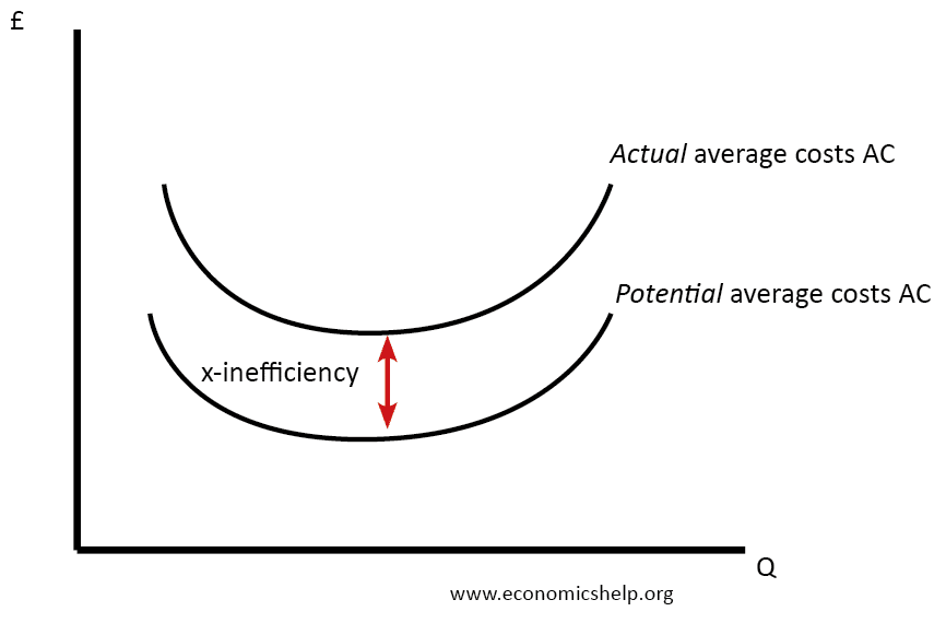
x-inefficiency

Comments

Popular posts from this blog

Income elasticity of demand (YED)

    Income elasticity of demand (YED)         % D QD/% D Y             Income elasticity of demand (YED): the responsiveness of the quantity demanded of a good to changes in consumer income. YED allows us to work out which goods are inferior, luxury and normal. When YED > 1 or <-1, demand is elastic. When YED is between -1 and 1, demand is inelastic. When YED < 0, goods/services are inferior. This means as income rises, demand for these goods decreases. (e.g. bus tickets) They vary inversely with income. When YED < -1, goods are very inferior (e.g. own-brand labels, cheap cuts of meat). When YED = 0, demand for the good is independent of income. When YED > 0, goods/services are normal. Demand for these goods vary directly with income, and the state of the economy. When YED is between 0 and 1, goods/services are necessary. When income increases, demand for these goods go up a proportional...

The Philips curve

The Philips curve  The Philips curve suggests a tradeoff between unemployment and inflation - to decrease unemployment, inflation has to rise. This creates a conflict between two macroeconomic objectives - targeting inflation at 2% (in the UK) and decreasing unemployment. 

PPF

Production Possibility Frontier Production Possibility Frontier (PPF): the curve showing the maximum combinations of goods or services that can be produced in a given time with available resources. Assumptions: -         Production over a specific time period like one year -         Inputs are fixed during this time period -         Technology doesn’t change during this time period ·        Meaning of points on and around the PPF—efficiency When you are on the PPF, you are working at maximum efficiency or full capacity. If you are within the PPF then you are under-utilising existing resources or resources are being used inefficiently. There is underemployment. The economy cannot produce past the frontier. Points outside the PPF are unattainable given the current inputs. ·        Causes and me...